Next: 18.3.2 Using shadowing model Up: 18.3 Shadowing model Previous: 18.3 Shadowing model Contents Index
The free space model and the two-ray model predict the received power
as a deterministic function of distance. They both represent the communication
range as an ideal circle. In reality, the received power at certain distance
is a random variable due to multipath propagation effects, which is also
known as fading effects. In fact, the above two models predicts the mean
received power at distance ![]() . A more general and widely-used model is
called the shadowing model [29].
. A more general and widely-used model is
called the shadowing model [29].
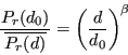
The shadowing model consists of two parts. The first one is known as path
loss model, which also predicts the mean received power at distance ![]() ,
denoted by
,
denoted by
![]() . It uses a close-in distance
. It uses a close-in distance ![]() as
a reference.
as
a reference.
![]() is computed relative to
is computed relative to ![]() as follows.
as follows.
![]() is called the path loss exponent, and is usually empirically
determined by field measurement. From Eqn. (18.1) we
know that
is called the path loss exponent, and is usually empirically
determined by field measurement. From Eqn. (18.1) we
know that ![]() for free space propagation. Table 18.1
gives some typical values of
for free space propagation. Table 18.1
gives some typical values of ![]() .
Larger values correspond to more obstructions and hence faster
decrease in average received power as distance becomes larger.
.
Larger values correspond to more obstructions and hence faster
decrease in average received power as distance becomes larger. ![]() can be computed from Eqn. (18.1).
can be computed from Eqn. (18.1).
The path loss is usually measured in dB. So from Eqn. (18.4) we have
The second part of the shadowing model reflects the variation of the received power at certain distance. It is a log-normal random variable, that is, it is of Gaussian distribution if measured in dB. The overall shadowing model is represented by
where ![]() is a Gaussian random variable with zero mean and
standard deviation
is a Gaussian random variable with zero mean and
standard deviation ![]() .
. ![]() is called the
shadowing deviation, and is also obtained by measurement. Table
18.2 shows some typical values of
is called the
shadowing deviation, and is also obtained by measurement. Table
18.2 shows some typical values of ![]() . Eqn.
(18.6) is also known as a log-normal shadowing model.
. Eqn.
(18.6) is also known as a log-normal shadowing model.
The shadowing model extends the ideal circle model to a richer statistic model: nodes can only probabilistically communicate when near the edge of the communication range.
![\begin{displaymath}
{\left[ \frac{\overline{P_r(d)}}{P_r(d_0)} \right]}_{dB} =
-10 \beta \log \left( \frac{d}{d_0} \right)
\end{displaymath}](img92.png)